Supersonic inlet design and analysis
For Compressible Fluid Flow, I designed and analyzed a supersonic air intake that slows high-speed air before it reaches an engine's compressor, while minimizing pressure losses. I combined shock-relation calculations, CAD in SOLIDWORKS and CFD in ANSYS Fluent.
- Problem
- Slow a Mach 2.2 flow with enough compression and deceleration while maintaining high pressure recovery.
- My contribution
- I calculated Mach numbers and pressure changes by hand, modeled the geometry in SOLIDWORKS, and simulated the flow in ANSYS Fluent.
- Engineering decisions
- Inclined ramps compress and decelerate the flow through successive oblique shocks. I used first-order upwind discretization for stable shock capturing.
- Evidence
- The dimensioned geometry, solver settings, Mach and pressure contours, line plots and the oblique shock calculation.
- Outcome
- The simulated flow slows in steps through the ramps and accelerates through the expansion, in agreement with compressible flow theory.
- M₂ ≈ 1.88
- Analytical prediction of Mach number behind the first shock.
- p₂/p₁ ≈ 1.63
- Analytical prediction of the static pressure ratio across the first shock.
What I did
- Analytical modeling. Calculated Mach numbers and pressure changes with oblique- and normal-shock relations.
- Geometry design. Modeled the inlet and ramp geometries in SOLIDWORKS.
- CFD simulation. Used ANSYS Fluent to investigate compressible flow and shock-wave behavior.
- Design comparison. Evaluated ramp configurations and their effects on pressure recovery.
- Engineering analysis. Investigated the tradeoff between flow deceleration and stagnation-pressure losses.
Mach number field
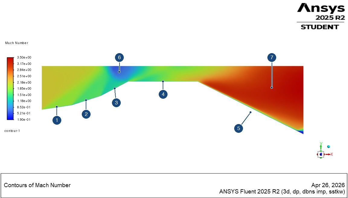
- 1: First ramp. A contour band starts at this ramp, the feature the analytical first-shock calculation addresses.
- 2: Second ramp. Mach number drops again as the wall turns further.
- 3: Third ramp, the steepest.
- 4: Flat section, below the region where the contour bands reach and cross.
- 5: Expansion. Mach number rises where the wall turns away.
- 6: Low-Mach pocket at the upper wall, above the end of the third ramp.
- 7: Highest-Mach region, downstream in the expansion.
Geometry
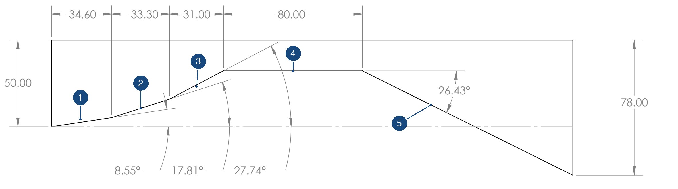
- 1: First ramp, 8.55°, starting at the inlet.
- 2: Second ramp, 17.81°.
- 3: Third ramp, 27.74°.
- 4: 80 mm flat section.
- 5: Expansion, where the wall drops away at 26.43°.
Solver setup
“Solver type: Density-based. Flow type: Steady, compressible. Energy equation: Enabled. Turbulence model: k-ω SST. Spatial discretization: First-order upwind for stable shock-capturing.”
“Inlet: Pressure far-field. Mach number: 2.2. Outlet: Pressure outlet. Walls: No-slip, adiabatic.”
“A structured mesh was generated with refinement near the geometry to capture shock structures.”
Analytical prediction of the first shock
I solved the first ramp by hand with the oblique shock relation, using M1 = 2.2, γ = 1.4 and θ = 8.55°:
tan θ = 2 cot β (M12 sin2 β − 1) / (M12 (γ + cos 2β) + 2)
The weak-shock solution is β ≈ 34.35°, which gives a normal Mach number of about 1.24. The normal shock relations then give M2 ≈ 1.88 and p2/p1 ≈ 1.63.
Simulation results
The flow slows through the ramps, then speeds up sharply through the expansion. The strongest compression is at the upper wall above the end of the third ramp, where the contours show a pocket of low Mach number and the highest pressure in the domain.
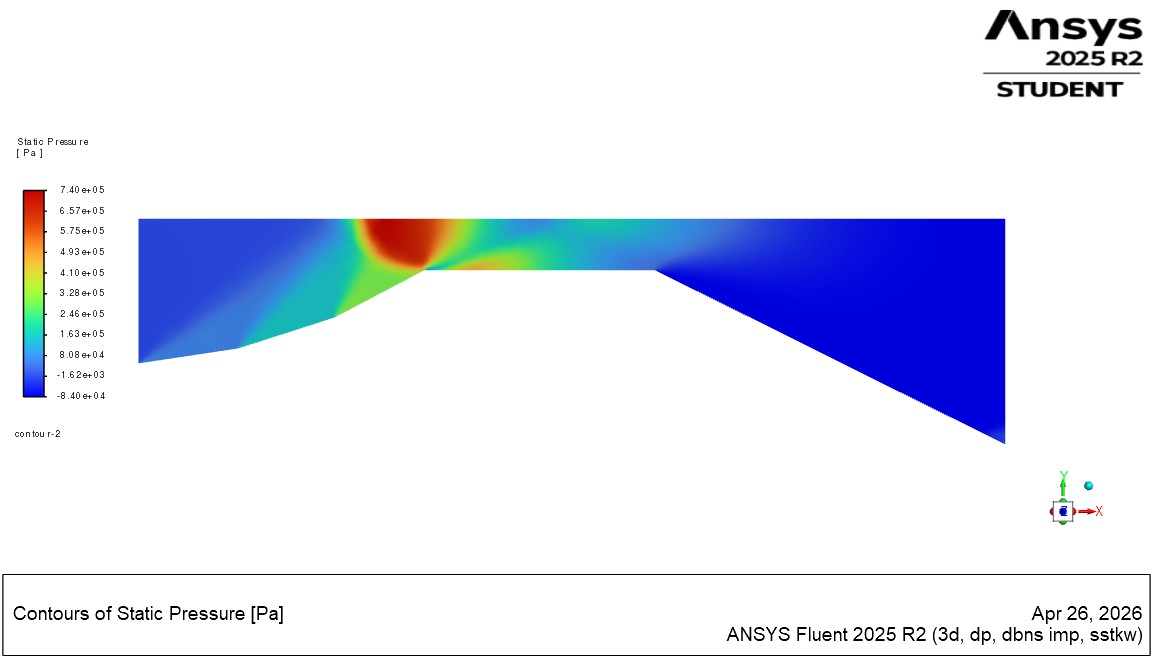
The two plots below sample one Fluent line through the flow, labeled line-7, with position running from about 0.01 to 0.075 m.
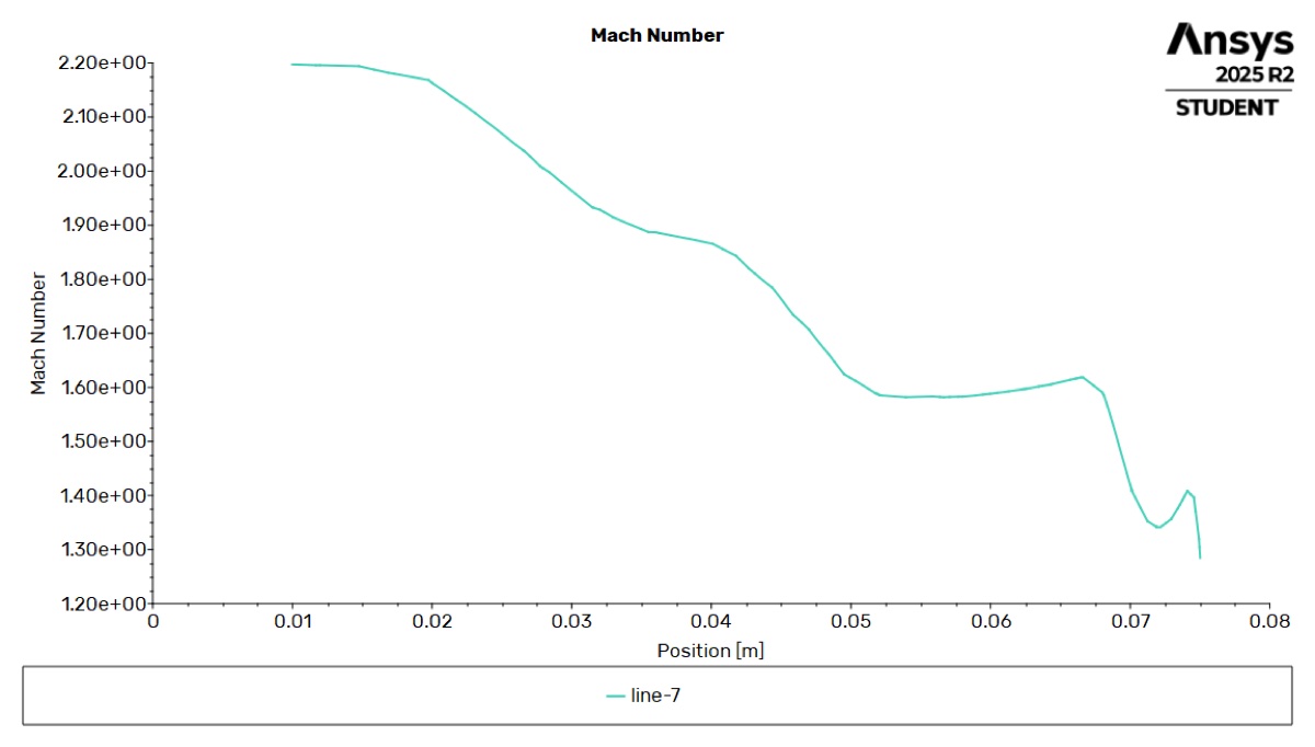
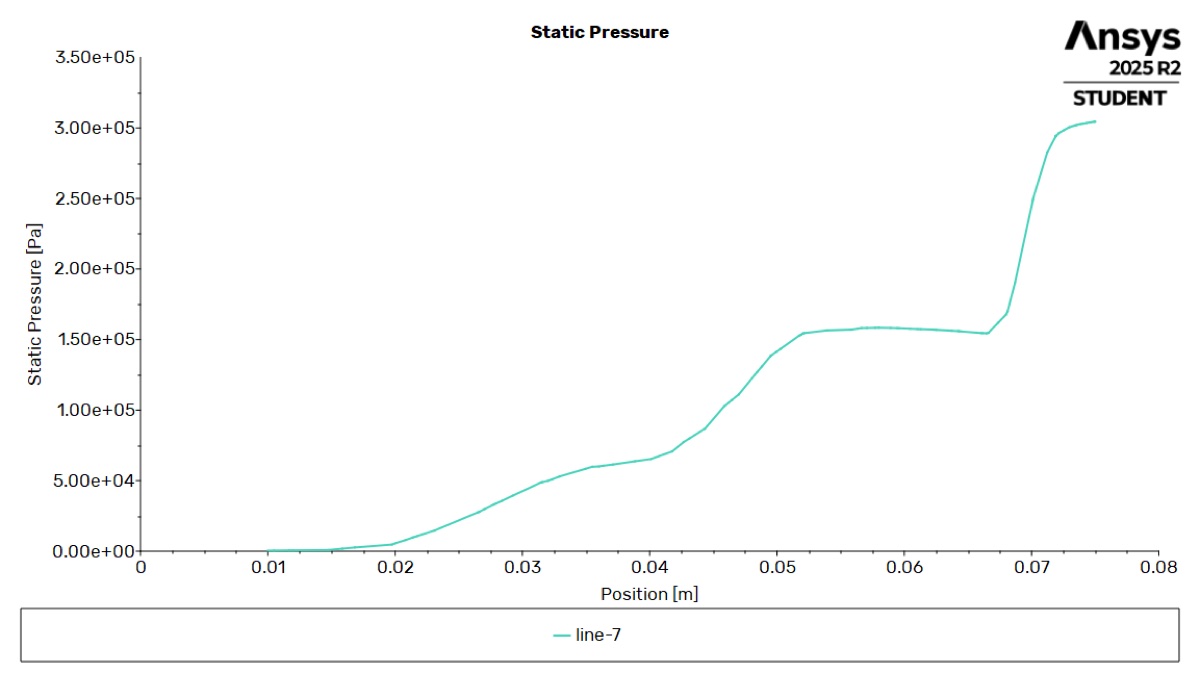
Mach number falls and pressure rises in steps along the line, which is the behavior compressible flow theory predicts.
Source file
- Supersonic inlet: geometry drawing
One-page SOLIDWORKS drawing of the geometry, with dimensions in millimeters.